4 Data Transformation

“Happy families are all alike; every unhappy family is unhappy in its own way.”

— Leo Tolstoy

“Tidy datasets are all alike, but every messy dataset is messy in its own way.”

— Hadley Wickham

First off…

Advanced R Challenges

This challenge is to understand and use this function to read in a series of csv files and transform them into one data.frame.


#Joel's awesome function

combineCSV <- function(fPath){ #see the r base cheatsheet for function syntax
  # List all files in the path
  f <- list.files(path = fPath, recursive = TRUE) #see ?list.files
  
  #separate files list and place into tibble (This is all the names and subids in the titles of the files)
  f_split <- as_tibble(str_split(f, "_|/", simplify = TRUE)) %>% #see ?str_split from stringr package, separated by "_"
    mutate(.id = row_number()) %>% #How does making a row number column help this process?
    select(".id", everything()) #How does everything() work?
  
  #read in all files to list
  fls <- lapply(str_c(fPath, f), read.csv, header = FALSE) #see ?str_c from stringr and ?lapply from the apply family
  
  #convert list to data frame
  d <- as.data.frame(rbindlist(fls, fill = TRUE, idcol = TRUE)) #see ?rbind_list from the data.table package
  
  #join data with identifying information
  e <- f_split %>% #Join df of names and ids with df of data
    full_join(d, by = ".id") #See ?full_join
}

Data Transformation with Dplyr

First, we clean the environment and get the tidyverse, which has dplyr.

rm(list = ls())
library(tidyverse)
#> ── Attaching packages ─────────────────────────────────────── tidyverse 1.3.1 ──
#> ✓ ggplot2 3.3.5     ✓ purrr   0.3.4
#> ✓ tibble  3.1.6     ✓ dplyr   1.0.7
#> ✓ tidyr   1.1.3     ✓ stringr 1.4.0
#> ✓ readr   1.4.0     ✓ forcats 0.5.1
#> ── Conflicts ────────────────────────────────────────── tidyverse_conflicts() ──
#> x dplyr::filter() masks stats::filter()
#> x dplyr::lag()    masks stats::lag()

4.1 Get a dataset from your .RData file

load('data/ready.RData')

ready.Rdata has multiple dataframes within it. This is the helpful thing about .RData files. They can contain all of the dataframes you need for a project or analysis.

df <- as_tibble(ccolor %>%
  select(subject = s, congruency = con, stimulus =S,
          response = R, reactionTime = RT))


tbl_df(ccolor) #Converts data to tbl class - Easier to view
#> Warning: `tbl_df()` was deprecated in dplyr 1.0.0.
#> Please use `tibble::as_tibble()` instead.
#> This warning is displayed once every 8 hours.
#> Call `lifecycle::last_lifecycle_warnings()` to see where this warning was generated.
#> # A tibble: 6,400 × 5
#>   s     con         S     R        RT
#>   <fct> <chr>       <fct> <chr> <dbl>
#> 1 1     congruent   blue  blue   1023
#> 2 1     incongruent blue  red     665
#> 3 1     congruent   red   red    1568
#> 4 1     congruent   blue  blue    955
#> 5 1     incongruent red   blue    792
#> 6 1     congruent   red   red     452
#> # … with 6,394 more rows

You can compare the classes…

class(ccolor)
#> [1] "data.frame"
class(tbl_df(ccolor))
#> [1] "tbl_df"     "tbl"        "data.frame"

or get a glimpse of the data…

glimpse(ccolor) #Gives the same information as clicking the blue circle in the environment panel
#> Rows: 6,400
#> Columns: 5
#> $ s   <fct> 1, 1, 1, 1, 1, 1, 1, 1, 1, 1, 1, 1, 1, 1, 1, 1, 1, 1, 1, 1, 1, 1, …
#> $ con <chr> "congruent", "incongruent", "congruent", "congruent", "incongruent…
#> $ S   <fct> blue, blue, red, blue, red, red, blue, red, blue, red, blue, blue,…
#> $ R   <chr> "blue", "red", "red", "blue", "blue", "red", "blue", "red", "blue"…
#> $ RT  <dbl> 1023, 665, 1568, 955, 792, 452, 369, 1067, 414, 763, 766, 563, 115…

or get the full thing…

View(ccolor) #Gives you a navigable display

4.2 Introduction to “The Pipe”

The pipe, aka %>%, takes you a level into the data, so…


ccolor %>%
  summarise(count = n()) # is the same as...
#>   count
#> 1  6400

summarise(ccolor, count = n())
#>   count
#> 1  6400

Now let’s do some descriptives…

ccolor %>%
  group_by(s) %>%
  summarise(count = n()) 
#> # A tibble: 20 × 2
#>   s     count
#>   <fct> <int>
#> 1 1       320
#> 2 2       320
#> 3 3       320
#> 4 4       320
#> 5 5       320
#> 6 6       320
#> # ℹ 14 more rows

# (Harder to read long, so we can spread it out)

ccolor %>%
  group_by(s) %>%
  summarise(count = n()) %>% #Let's name this something easy to type and remember, like "count"
  pivot_wider(names_from = s, values_from = count)
#> # A tibble: 1 × 20
#>     `1`   `2`   `3`   `4`   `5`   `6`   `7`   `8`   `9`  `10`  `11`  `12`  `13`
#>   <int> <int> <int> <int> <int> <int> <int> <int> <int> <int> <int> <int> <int>
#> 1   320   320   320   320   320   320   320   320   320   320   320   320   320
#> # ℹ 7 more variables: `14` <int>, `15` <int>, `16` <int>, `17` <int>,
#> #   `18` <int>, `19` <int>, `20` <int>

We can also wrap functions around the whole data object…

as.matrix(ccolor %>%
  group_by(s) %>%
  summarise(count = n()) %>%
  pivot_wider(names_from = s, values_from = count)) #or we can subset it
#>        1   2   3   4   5   6   7   8   9  10  11  12  13  14  15  16  17  18
#> [1,] 320 320 320 320 320 320 320 320 320 320 320 320 320 320 320 320 320 320
#>       19  20
#> [1,] 320 320

data.frame(ccolor %>%
  group_by(s) %>%
  summarise(count = n()) %>%
  pivot_wider(names_from = s, values_from = count))[,4:7]
#>    X4  X5  X6  X7
#> 1 320 320 320 320

What happened to the names? What is that X4, X5, stuff? That’s what R does when it doesn’t know the column names, but in this case it actually does. Check with colnames()

colnames(ccolor %>%
           group_by(s) %>%
           summarise(count = n()) %>% #Let's name this something easy to type and remember, like "count"
           pivot_wider(names_from = s, values_from = count))
#>  [1] "1"  "2"  "3"  "4"  "5"  "6"  "7"  "8"  "9"  "10" "11" "12" "13" "14" "15"
#> [16] "16" "17" "18" "19" "20"

None of these changes are being saved! You can make new objects with the <- operator.

df <- ccolor #do some stuff here

Above I used group_by(s), which groups by participant, summarise() with n(), which counts the number of rows, and pivot_wider(), which takes the column s, turns each row into a column, and puts the value argument in that column.

There’s also filter(), gather(), separate(), unite(), select(), distinct(), sample_n(), slice(), and many more.

For example:

as_tibble(ccolor %>%
  filter(s == 1))# "==" is a logic operator, which works with most classes of data
#> # A tibble: 320 × 5
#>   s     con         S     R        RT
#>   <fct> <chr>       <fct> <chr> <dbl>
#> 1 1     congruent   blue  blue   1023
#> 2 1     incongruent blue  red     665
#> 3 1     congruent   red   red    1568
#> 4 1     congruent   blue  blue    955
#> 5 1     incongruent red   blue    792
#> 6 1     congruent   red   red     452
#> # … with 314 more rows

class(ccolor$s)
#> [1] "factor"

4.3 Aside on the apply family

<ASIDE> - for those of you interested in replacing your For Loops, this is how you’d do it. Here’s a quick introduction to the apply family. We can apply class() to muliple columns.

Say we want to get the class of every column…

apply(ccolor, MARGIN = 2, FUN = class) #Something about changing it to an array loses its class attributes
#>           s         con           S           R          RT 
#> "character" "character" "character" "character" "character"
lapply(ccolor, FUN = class) #list apply makes the output of the call a list
#> $s
#> [1] "factor"
#> 
#> $con
#> [1] "character"
#> 
#> $S
#> [1] "factor"
#> 
#> $R
#> [1] "character"
#> 
#> $RT
#> [1] "numeric"
sapply(ccolor,FUN = class) #simple apply tries to output the simplest outcome
#>           s         con           S           R          RT 
#>    "factor" "character"    "factor" "character"   "numeric"

The bottom two assume you mean the columns, while the top one you have to specify. tapply is different, because you index (or group) by another variable. Say we want mean RT by subject…

tapply(X = ccolor$RT, INDEX = ccolor$s, FUN = mean) #We'd do it like that.
#>    1    2    3    4    5    6    7    8    9   10   11   12   13   14   15   16 
#>  790  731  485  847  824  536 1065 1325 1090 1002  840  914  900 1012  953   NA 
#>   17   18   19   20 
#>  996  980  719  623

mapply stands for “multivariate apply’, and works like this:

# Create a 4x4 matrix
Q1 <- matrix(c(rep(1, 4), rep(2, 4), rep(3, 4), rep(4, 4)),4,4)
Q1 #Or you could use mapply()
#>      [,1] [,2] [,3] [,4]
#> [1,]    1    2    3    4
#> [2,]    1    2    3    4
#> [3,]    1    2    3    4
#> [4,]    1    2    3    4
mapply(rep, 1:4,4) #repeat 1 through 4, 4 times
#>      [,1] [,2] [,3] [,4]
#> [1,]    1    2    3    4
#> [2,]    1    2    3    4
#> [3,]    1    2    3    4
#> [4,]    1    2    3    4

Say you want to mean-center some data

dataPoints <- matrix(rnorm(30), nrow=5, ncol=6)

Find means per column with apply()

dataPoints_means <- apply(dataPoints, 2, mean) #Margin = 2 signifies "do it to the columns"

Find standard deviation with apply()

dataPoints_sdev <- apply(dataPoints, 2, sd)

Center the points

dataPoints_Trans1 <- sweep(dataPoints, 2, dataPoints_means,"-") #subtract mean from points in columns

Return the result

dataPoints_Trans1
#>        [,1]     [,2]   [,3]    [,4]    [,5]   [,6]
#> [1,] -0.807  1.43794 -0.758 -1.3013  0.0376  0.580
#> [2,]  0.849 -1.53229  0.425  0.0397 -0.0676 -0.258
#> [3,] -1.844  0.04220  1.861  0.5091 -1.7351  0.662
#> [4,]  0.588  0.04533 -1.835  1.1047  0.3072 -0.149
#> [5,]  1.215  0.00682  0.308 -0.3523  1.4579 -0.835

Normalize

dataPoints_Trans2 <- sweep(dataPoints_Trans1, 2, dataPoints_sdev, "/") #divide new point values by standard deviation in columns

Return the result

dataPoints_Trans2
#>        [,1]     [,2]   [,3]    [,4]    [,5]   [,6]
#> [1,] -0.628  1.36800 -0.547 -1.4329  0.0328  0.929
#> [2,]  0.661 -1.45776  0.306  0.0437 -0.0591 -0.413
#> [3,] -1.436  0.04015  1.343  0.5607 -1.5165  1.060
#> [4,]  0.458  0.04312 -1.325  1.2165  0.2685 -0.239
#> [5,]  0.946  0.00649  0.222 -0.3880  1.2742 -1.337

Now you have mean-centered data points, probably for a regression model.

</ASIDE>

4.4 Extracting rows

One thing we always want to do is extract rows based on some criteria. For example, in Reaction Time data we often trim the early responses as anticipatory, and the late responses as outliers.

Challenge 1: Find and remove the rows with NAs, save it out to “newdf”

newdf <- ...

Challenge 2: Filter out RT’s below 150 milliseconds and show how many you’ve filtered out.

newdf %>%
  filter(...) %>%
  summarise(...)

Challenge 3: Get the number of observations (rows) kept and removed with group_by()

newdf %>%
  group_by(...) %>%
  summarise(...)

In papers, you want to report the proportion of data you have removed and the criteria with which you removed that data.

Now you have the slow responses, but a more appropriate standard might be removing data above three standard deviations from the mean for each participant’s own distribution. Let’s try that now…

newdf %>% #Step 1 is to group by the subject and get the mean and sd
  group_by(s) %>%
  mutate(mRT = mean(RT), RTsd = sd(RT))
#> # A tibble: 6,399 × 7
#> # Groups:   s [20]
#>   s     con         S     R        RT   mRT  RTsd
#>   <fct> <chr>       <fct> <chr> <dbl> <dbl> <dbl>
#> 1 1     congruent   blue  blue   1023  790.  775.
#> 2 1     incongruent blue  red     665  790.  775.
#> 3 1     congruent   red   red    1568  790.  775.
#> 4 1     congruent   blue  blue    955  790.  775.
#> 5 1     incongruent red   blue    792  790.  775.
#> 6 1     congruent   red   red     452  790.  775.
#> # ℹ 6,393 more rows

newdf %>% #Step 2 is to make a cutoff 3 standard deviations above the mean for each participant
  group_by(s) %>%
  mutate(mRT = mean(RT), RTsd = sd(RT)) %>%
  mutate(cutoff = mRT + 3*RTsd)
#> # A tibble: 6,399 × 8
#> # Groups:   s [20]
#>   s     con         S     R        RT   mRT  RTsd cutoff
#>   <fct> <chr>       <fct> <chr> <dbl> <dbl> <dbl>  <dbl>
#> 1 1     congruent   blue  blue   1023  790.  775.  3115.
#> 2 1     incongruent blue  red     665  790.  775.  3115.
#> 3 1     congruent   red   red    1568  790.  775.  3115.
#> 4 1     congruent   blue  blue    955  790.  775.  3115.
#> 5 1     incongruent red   blue    792  790.  775.  3115.
#> 6 1     congruent   red   red     452  790.  775.  3115.
#> # ℹ 6,393 more rows


newdf %>% #Step 3 Let's clean up the columns we need and the ones we don't
  group_by(s) %>%
  mutate(mRT = mean(RT), RTsd = sd(RT)) %>%
  mutate(cutoff = mRT + 3*RTsd) %>%
  select(-mRT, -RTsd)
#> # A tibble: 6,399 × 6
#> # Groups:   s [20]
#>   s     con         S     R        RT cutoff
#>   <fct> <chr>       <fct> <chr> <dbl>  <dbl>
#> 1 1     congruent   blue  blue   1023  3115.
#> 2 1     incongruent blue  red     665  3115.
#> 3 1     congruent   red   red    1568  3115.
#> 4 1     congruent   blue  blue    955  3115.
#> 5 1     incongruent red   blue    792  3115.
#> 6 1     congruent   red   red     452  3115.
#> # ℹ 6,393 more rows


newdf %>% #Step 4 Now let's filter those RTs above the cutoff and count them
  group_by(s) %>%
  mutate(mRT = mean(RT), RTsd = sd(RT)) %>%
  mutate(cutoff = mRT + 3*RTsd) %>%
  select(-mRT, -RTsd) %>%
  filter(RT > cutoff) %>%
  summarise(n = n()) %>% #spread it out so its easy to read
  pivot_wider(names_from = s, values_from = n)
#> # A tibble: 1 × 20
#>     `1`   `2`   `3`   `4`   `5`   `6`   `7`   `8`   `9`  `10`  `11`  `12`  `13`
#>   <int> <int> <int> <int> <int> <int> <int> <int> <int> <int> <int> <int> <int>
#> 1     4     4     4     4     7     6     6     3     8     5     1     7     4
#> # ℹ 7 more variables: `14` <int>, `15` <int>, `16` <int>, `17` <int>,
#> #   `18` <int>, `19` <int>, `20` <int>


newdf %>% #We can see the proportion of removed data
  group_by(s) %>%
  mutate(mRT = mean(RT), RTsd = sd(RT)) %>%
  mutate(cutoff = mRT + 3*RTsd) %>%
  select(-mRT, -RTsd) %>%
  group_by(RT > cutoff | RT < 150) %>%
  summarise(n = n()) %>%
  mutate(prop = (n/sum(n))*100)
#> # A tibble: 2 × 3
#>   `RT > cutoff | RT < 150`     n  prop
#>   <lgl>                    <int> <dbl>
#> 1 FALSE                     6289 98.3 
#> 2 TRUE                       110  1.72

dfclean <- newdf %>% #Save it out as dfclean
  group_by(s) %>%
  mutate(mRT = mean(RT), RTsd = sd(RT)) %>%
  mutate(cutoff = mRT + 3*RTsd) %>%
  select(-mRT, -RTsd) %>%
  filter(RT < cutoff & RT > 150) #The RTs must be less than the cutoff AND greater than 150 ms

Now we’re ready to do some descriptive statistics with the groups

Challenge 4: What is the mean reaction time and standard deviation for congruent vs incongruent trials

#hint group_by(the factor you're interested in)
dfclean %>%
  group_by(...) %>%
  summarise(...)

Challenge 5: Get the mean and sd of participant means for congruent vs incongruent trials and compare to the previous outcome.

dfclean %>%
  group_by(...) %>%
  summarise(...) %>%
  group_by(...) %>%
  summarise(..., ...)

This is a quirk of repeated measures fully within designs, as the levels of analysis are nested. More on that later. We can quickly visualize some of these things, like the distribution of responses in base R. Note: Soon we will learn to visualize everything in ggplot2.

hist(dfclean$RT, breaks = 100)

#Add a line for the mean
hist(dfclean$RT, breaks = 100)
abline(v = mean(dfclean$RT),
       col = "red",
       lwd = 2)
#add a line for the median
abline(v = median(dfclean$RT),
       col = "blue",
       lwd = 3)
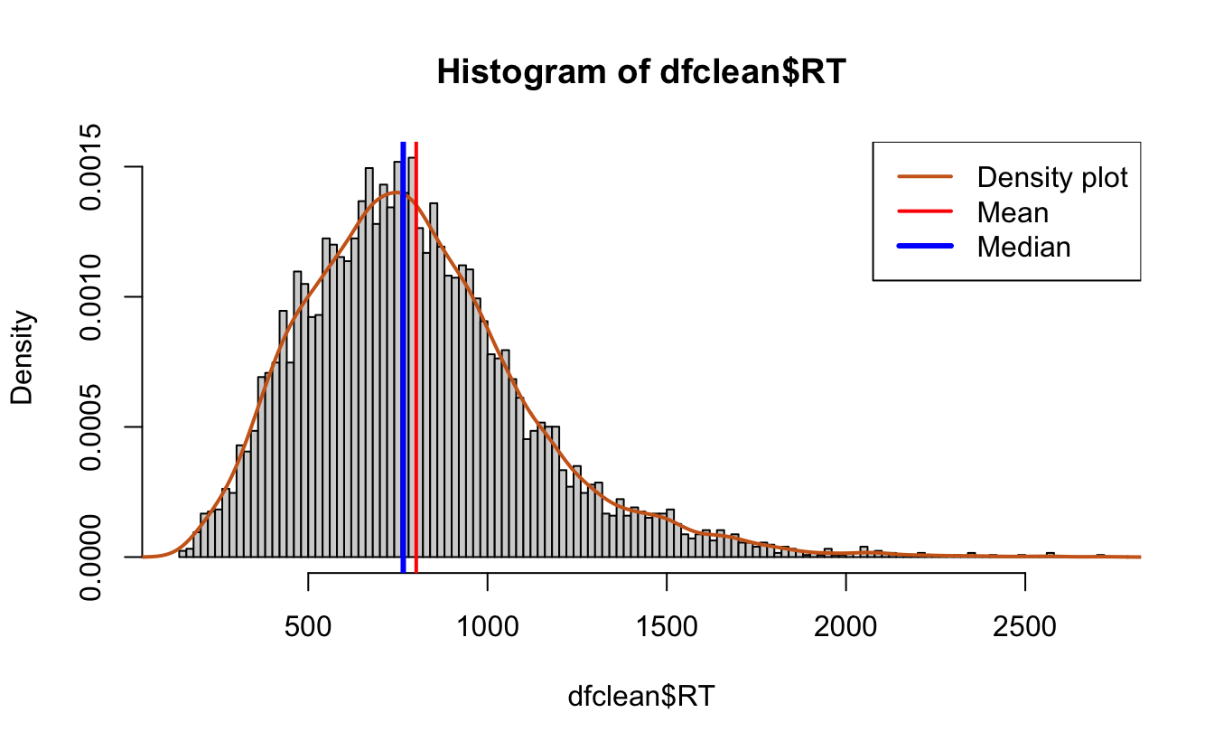
lines(density(dfclean$RT),
      lwd = 2, # thickness of line
      col = "chocolate3")# density plot

#Add a density plot,
hist(dfclean$RT, breaks = 100,
     prob = T)
lines(density(dfclean$RT),
      lwd = 2, # thickness of line
      col = "chocolate3")# density plot
abline(v = mean(dfclean$RT),
       col = "red",
       lwd = 2)
#add a line for the median
abline(v = median(dfclean$RT),
       col = "blue",
       lwd = 3)

legend(x = "topright", # location of legend within plot area
       c("Density plot", "Mean", "Median"),
       col = c("chocolate3", "red", "blue"),
       lwd = c(2, 2, 3))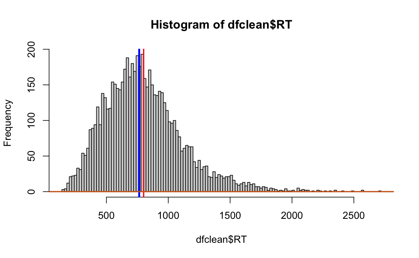

4.5 Pivoting, Separating and Uniting

look at this tibble(data.frame)

stocks <- tibble(
  year   = c(2015, 2015, 2016, 2016),
  half  = c(   1,    2,     1,    2),
  return = c(1.88, 0.59, 0.92, 0.17)
)

pivot_longer and pivot_wider are not opposites.


stocks %>%
  pivot_wider(names_from = "year",values_from = "return") %>%
  pivot_longer(cols = `2015`:`2016`,names_to = "year")
#> # A tibble: 4 × 3
#>    half year  value
#>   <dbl> <chr> <dbl>
#> 1     1 2015   1.88
#> 2     1 2016   0.92
#> 3     2 2015   0.59
#> 4     2 2016   0.17

You can make data.frames with space using the tribble() function

people <- tribble(
  ~name,             ~key,    ~value,
  #-----------------|--------|------
  "Phillip Woods",   "age",       45,
  "Phillip Woods",   "height",   186,
  "Jessica Cordero", "age",       37,
  "Jessica Cordero", "height",   156
)

people
#> # A tibble: 4 × 3
#>   name            key    value
#>   <chr>           <chr>  <dbl>
#> 1 Phillip Woods   age       45
#> 2 Phillip Woods   height   186
#> 3 Jessica Cordero age       37
#> 4 Jessica Cordero height   156

Challenge 6: spread people so height and age have their own column


newpeople <- people %>%
  pivot_wider(...)

Challenge 7: gather newpeople so that height and age are back together


newpeople %>%
  pivot_longer(...)

You can separate or unite columns based upon a separator

people %>%
  separate(name, into = c("first","last"))
#> # A tibble: 4 × 4
#>   first   last    key    value
#>   <chr>   <chr>   <chr>  <dbl>
#> 1 Phillip Woods   age       45
#> 2 Phillip Woods   height   186
#> 3 Jessica Cordero age       37
#> 4 Jessica Cordero height   156

How did it know? We usually have to specify the separator

weirdpeople <- people %>%
  separate(name, into = c("befored","afterd"), sep = "d")

Notice that the separator disappears

Challenge 8: Unite the two columns above with “d” as a separator

weirdpeople %>%
  unite(...)

That’s a lot to take in, so we’ll do questions about this content or queries about how to accomplish different data transformations.

4.6 Solutions to Challenges